17.2: Bayesian Hypothesis Tests

• Danielle Navarro
• University of New South Wales

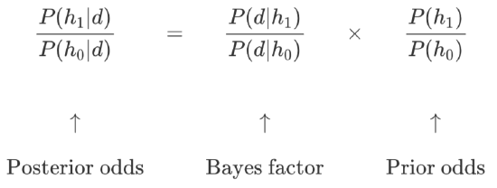
In Chapter 11 I described the orthodox approach to hypothesis testing. It took an entire chapter to describe, because null hypothesis testing is a very elaborate contraption that people find very hard to make sense of. In contrast, the Bayesian approach to hypothesis testing is incredibly simple. Let’s pick a setting that is closely analogous to the orthodox scenario. There are two hypotheses that we want to compare, a null hypothesis h₀ and an alternative hypothesis h₁. Prior to running the experiment we have some beliefs P(h) about which hypotheses are true. We run an experiment and obtain data d. Unlike frequentist statistics Bayesian statistics does allow to talk about the probability that the null hypothesis is true. Better yet, it allows us to calculate the posterior probability of the null hypothesis, using Bayes’ rule: \(\ P(h_0 | d) = \dfrac\) This formula tells us exactly how much belief we should have in the null hypothesis after having observed the data d. Similarly, we can work out how much belief to place in the alternative hypothesis using essentially the same equation. All we do is change the subscript: \(\ P(h_1 | d) = \dfrac\) It’s all so simple that I feel like an idiot even bothering to write these equations down, since all I’m doing is copying Bayes rule from the previous section. 259

Bayes factor

In practice, most Bayesian data analysts tend not to talk in terms of the raw posterior probabilities P(h₀|d) and P(h₁|d). Instead, we tend to talk in terms of the posterior odds ratio. Think of it like betting. Suppose, for instance, the posterior probability of the null hypothesis is 25%, and the posterior probability of the alternative is 75%. The alternative hypothesis is three times as probable as the null, so we say that the odds are 3:1 in favour of the alternative. Mathematically, all we have to do to calculate the posterior odds is divide one posterior probability by the other: \(\ \dfrac=\dfrac=3\) Or, to write the same thing in terms of the equations above: \(\ \dfrac = \dfrac \times \dfrac\) Actually, this equation is worth expanding on. There are three different terms here that you should know. On the left hand side, we have the posterior odds, which tells you what you believe about the relative plausibilty of the null hypothesis and the alternative hypothesis after seeing the data. On the right hand side, we have the prior odds, which indicates what you thought before seeing the data. In the middle, we have the Bayes factor, which describes the amount of evidence provided by the data: The Bayes factor (sometimes abbreviated as BF) has a special place in the Bayesian hypothesis testing, because it serves a similar role to the p-value in orthodox hypothesis testing: it quantifies the strength of evidence provided by the data, and as such it is the Bayes factor that people tend to report when running a Bayesian hypothesis test. The reason for reporting Bayes factors rather than posterior odds is that different researchers will have different priors. Some people might have a strong bias to believe the null hypothesis is true, others might have a strong bias to believe it is false. Because of this, the polite thing for an applied researcher to do is report the Bayes factor. That way, anyone reading the paper can multiply the Bayes factor by their own personal prior odds, and they can work out for themselves what the posterior odds would be. In any case, by convention we like to pretend that we give equal consideration to both the null hypothesis and the alternative, in which case the prior odds equals 1, and the posterior odds becomes the same as the Bayes factor.

Interpreting Bayes factors

One of the really nice things about the Bayes factor is the numbers are inherently meaningful. If you run an experiment and you compute a Bayes factor of 4, it means that the evidence provided by your data corresponds to betting odds of 4:1 in favour of the alternative. However, there have been some attempts to quantify the standards of evidence that would be considered meaningful in a scientific context. The two most widely used are from Jeffreys (1961) and Kass and Raftery (1995). Of the two, I tend to prefer the Kass and Raftery (1995) table because it’s a bit more conservative. So here it is:

And to be perfectly honest, I think that even the Kass and Raftery standards are being a bit charitable. If it were up to me, I’d have called the “positive evidence” category “weak evidence”. To me, anything in the range 3:1 to 20:1 is “weak” or “modest” evidence at best. But there are no hard and fast rules here: what counts as strong or weak evidence depends entirely on how conservative you are, and upon the standards that your community insists upon before it is willing to label a finding as “true”. In any case, note that all the numbers listed above make sense if the Bayes factor is greater than 1 (i.e., the evidence favours the alternative hypothesis). However, one big practical advantage of the Bayesian approach relative to the orthodox approach is that it also allows you to quantify evidence for the null. When that happens, the Bayes factor will be less than 1. You can choose to report a Bayes factor less than 1, but to be honest I find it confusing. For example, suppose that the likelihood of the data under the null hypothesis P(d|h₀) is equal to 0.2, and the corresponding likelihood P(d|h₀) under the alternative hypothesis is 0.1. Using the equations given above, Bayes factor here would be: \(\ BF=\dfrac=\dfrac=0.5\) Read literally, this result tells is that the evidence in favour of the alternative is 0.5 to 1. I find this hard to understand. To me, it makes a lot more sense to turn the equation “upside down”, and report the amount op evidence in favour of the null. In other words, what we calculate is this: \(\ BF^ <\prime>= \dfrac=\dfrac=2\) And what we would report is a Bayes factor of 2:1 in favour of the null. Much easier to understand, and you can interpret this using the table above.

This page titled 17.2: Bayesian Hypothesis Tests is shared under a CC BY-SA 4.0 license and was authored, remixed, and/or curated by Danielle Navarro via source content that was edited to the style and standards of the LibreTexts platform.

1. Back to top
2. • 17.1: Probabilistic Reasoning by Rational Agents
   • 17.3: Why Be a Bayesian?

• Was this article helpful?
• Yes
• No